Explain tensorflow model using Shap and model Weights on METABRIC data
from platform import python_version
python_version()'3.8.18'import numpy as np
import pandas as pd
import sklearn
import matplotlib.pyplot as plt
from sklearn.model_selection import GridSearchCV
from sklearn.model_selection import train_test_split
from sklearn.preprocessing import MinMaxScaler
from sklearn.metrics import confusion_matrix,ConfusionMatrixDisplay
import tensorflow as tf
from tensorflow import keras
from tensorflow.keras.layers import Dense, Dropout
from tensorflow.keras.callbacks import EarlyStopping
from tensorflow.keras.models import Sequential
from keras import regularizers
import shap
# Check for TensorFlow GPU access
print(f"TensorFlow has access to the following devices:\n{tf.config.list_physical_devices()}")
# See TensorFlow version
print(f"TensorFlow version: {tf.__version__}")TensorFlow has access to the following devices:
[PhysicalDevice(name='/physical_device:CPU:0', device_type='CPU'), PhysicalDevice(name='/physical_device:GPU:0', device_type='GPU')]
TensorFlow version: 2.13.0tf.test.is_gpu_available()2024-02-21 14:06:44.743687: I tensorflow/core/common_runtime/pluggable_device/pluggable_device_factory.cc:303] Could not identify NUMA node of platform GPU ID 0, defaulting to 0. Your kernel may not have been built with NUMA support.
2024-02-21 14:06:44.743733: I tensorflow/core/common_runtime/pluggable_device/pluggable_device_factory.cc:269] Created TensorFlow device (/device:GPU:0 with 0 MB memory) -> physical PluggableDevice (device: 0, name: METAL, pci bus id: <undefined>)
TrueData loading and preprocessing
Expression data
metabric_X = "https://raw.githubusercontent.com/LamineTourelab/Tutorial/main/Data/metabric_test.csv"
df = pd.read_csv(metabric_X)
df.head(5)| CD52 | DARC | DCN | DB005376 | TAT | GSTM1 | UGT2B11 | AKR7A3 | SERHL2 | ASS1 | ... | MYB | PROM1 | GSTT1 | NELL2 | CST5 | CCL5 | TFF3 | CDH3 | SLC39A6 | SHISA2 | |
|---|---|---|---|---|---|---|---|---|---|---|---|---|---|---|---|---|---|---|---|---|---|
| 0 | 8.240128 | 10.731211 | 11.251592 | 5.350604 | 5.698745 | 5.626606 | 5.845062 | 8.334491 | 7.150713 | 9.887783 | ... | 7.864506 | 10.475799 | 5.236212 | 6.462909 | 5.333817 | 8.771015 | 10.545305 | 8.588759 | 8.287300 | 6.155340 |
| 1 | 7.441887 | 6.498731 | 9.968656 | 5.701508 | 5.416231 | 5.108180 | 5.382890 | 10.277779 | 6.070879 | 6.203103 | ... | 10.699097 | 5.977531 | 8.450049 | 7.486917 | 5.464502 | 8.216436 | 10.422146 | 5.838056 | 10.380559 | 9.409817 |
| 2 | 7.977708 | 6.615727 | 9.632207 | 6.346358 | 5.480066 | 5.356168 | 7.798285 | 9.117568 | 6.230590 | 7.928613 | ... | 9.861437 | 8.517411 | 7.230715 | 11.957439 | 5.359362 | 8.012079 | 12.201802 | 6.681570 | 10.009376 | 9.094121 |
| 3 | 8.045781 | 5.806614 | 8.927632 | 5.628718 | 5.746114 | 5.402901 | 6.043053 | 10.057702 | 11.682904 | 10.047193 | ... | 9.138474 | 9.099391 | 8.072639 | 12.478907 | 5.523048 | 9.245577 | 14.169804 | 6.392376 | 11.141299 | 10.039994 |
| 4 | 9.001653 | 7.928994 | 9.356798 | 5.484226 | 5.152513 | 5.401268 | 8.511554 | 11.127156 | 7.472530 | 7.200276 | ... | 9.591358 | 7.264378 | 8.975517 | 10.044922 | 5.034380 | 10.243518 | 13.568835 | 8.476834 | 8.916101 | 5.929184 |
5 rows × 295 columns
df.info()<class 'pandas.core.frame.DataFrame'>
RangeIndex: 1897 entries, 0 to 1896
Columns: 295 entries, CD52 to SHISA2
dtypes: float64(295)
memory usage: 4.3 MBdf.describe()| CD52 | DARC | DCN | DB005376 | TAT | GSTM1 | UGT2B11 | AKR7A3 | SERHL2 | ASS1 | ... | MYB | PROM1 | GSTT1 | NELL2 | CST5 | CCL5 | TFF3 | CDH3 | SLC39A6 | SHISA2 | |
|---|---|---|---|---|---|---|---|---|---|---|---|---|---|---|---|---|---|---|---|---|---|
| count | 1897.000000 | 1897.000000 | 1897.000000 | 1897.000000 | 1897.000000 | 1897.000000 | 1897.000000 | 1897.000000 | 1897.000000 | 1897.000000 | ... | 1897.000000 | 1897.000000 | 1897.000000 | 1897.000000 | 1897.000000 | 1897.000000 | 1897.000000 | 1897.000000 | 1897.000000 | 1897.000000 |
| mean | 8.522002 | 7.439279 | 8.592254 | 6.084079 | 6.267616 | 6.477882 | 6.920908 | 9.397352 | 7.558455 | 8.298495 | ... | 9.743111 | 8.041666 | 8.295523 | 7.466347 | 6.033271 | 9.845330 | 11.742209 | 7.465389 | 9.204424 | 7.725656 |
| std | 1.349624 | 1.323882 | 1.366120 | 1.489150 | 1.623607 | 1.490238 | 2.132190 | 1.280389 | 1.724598 | 1.314099 | ... | 1.242550 | 1.996117 | 1.691650 | 1.532031 | 1.500256 | 1.357065 | 2.444823 | 1.274105 | 1.620264 | 1.659966 |
| min | 5.018810 | 5.099984 | 5.074217 | 4.922326 | 4.925973 | 4.939510 | 4.988302 | 6.888636 | 5.214098 | 5.001618 | ... | 5.565536 | 5.047322 | 4.854543 | 5.030010 | 4.965204 | 5.685101 | 5.154748 | 5.103031 | 5.510203 | 5.119337 |
| 25% | 7.526147 | 6.337077 | 7.585572 | 5.315275 | 5.400663 | 5.428807 | 5.547688 | 8.359180 | 6.265815 | 7.277712 | ... | 9.072006 | 6.297426 | 7.469392 | 6.264153 | 5.337878 | 8.875585 | 10.657896 | 6.461509 | 7.869267 | 6.363869 |
| 50% | 8.448275 | 7.331663 | 8.608817 | 5.461374 | 5.563156 | 5.624529 | 5.881415 | 9.331409 | 7.083379 | 8.280220 | ... | 10.023695 | 7.623121 | 8.889979 | 7.056264 | 5.484401 | 9.857851 | 12.473404 | 7.303850 | 9.201048 | 7.358426 |
| 75% | 9.428863 | 8.370030 | 9.566763 | 5.971988 | 6.175448 | 7.490048 | 7.556015 | 10.241203 | 8.371308 | 9.256413 | ... | 10.654395 | 9.607842 | 9.489065 | 8.371956 | 5.818663 | 10.791775 | 13.588736 | 8.255375 | 10.508201 | 8.869039 |
| max | 13.374739 | 11.619202 | 12.478475 | 13.010996 | 13.166804 | 12.070735 | 14.145451 | 13.512971 | 13.731721 | 12.182876 | ... | 12.091906 | 13.569006 | 12.784519 | 13.110442 | 13.922840 | 14.004198 | 14.808641 | 12.003642 | 13.440167 | 12.874823 |
8 rows × 295 columns
Label data
metabric_y = "https://raw.githubusercontent.com/LamineTourelab/Tutorial/main/Data/metabric_clin.csv"
metadata = pd.read_csv(metabric_y)
metadata.head(5)| PATIENT_ID | LYMPH_NODES_EXAMINED_POSITIVE | NPI | CELLULARITY | CHEMOTHERAPY | COHORT | ER_IHC | HER2_SNP6 | HORMONE_THERAPY | INFERRED_MENOPAUSAL_STATE | ... | OS_STATUS | CLAUDIN_SUBTYPE | THREEGENE | VITAL_STATUS | LATERALITY | RADIO_THERAPY | HISTOLOGICAL_SUBTYPE | BREAST_SURGERY | RFS_STATUS | RFS_MONTHS | |
|---|---|---|---|---|---|---|---|---|---|---|---|---|---|---|---|---|---|---|---|---|---|
| 0 | MB-0000 | 10.0 | 6.044 | NaN | NO | 1.0 | Positve | NEUTRAL | YES | Post | ... | 0:LIVING | claudin-low | ER-/HER2- | Living | Right | YES | Ductal/NST | MASTECTOMY | 0:Not Recurred | 138.65 |
| 1 | MB-0002 | 0.0 | 4.020 | High | NO | 1.0 | Positve | NEUTRAL | YES | Pre | ... | 0:LIVING | LumA | ER+/HER2- High Prolif | Living | Right | YES | Ductal/NST | BREAST CONSERVING | 0:Not Recurred | 83.52 |
| 2 | MB-0005 | 1.0 | 4.030 | High | YES | 1.0 | Positve | NEUTRAL | YES | Pre | ... | 1:DECEASED | LumB | NaN | Died of Disease | Right | NO | Ductal/NST | MASTECTOMY | 1:Recurred | 151.28 |
| 3 | MB-0006 | 3.0 | 4.050 | Moderate | YES | 1.0 | Positve | NEUTRAL | YES | Pre | ... | 0:LIVING | LumB | NaN | Living | Right | YES | Mixed | MASTECTOMY | 0:Not Recurred | 162.76 |
| 4 | MB-0008 | 8.0 | 6.080 | High | YES | 1.0 | Positve | NEUTRAL | YES | Post | ... | 1:DECEASED | LumB | ER+/HER2- High Prolif | Died of Disease | Right | YES | Mixed | MASTECTOMY | 1:Recurred | 18.55 |
5 rows × 24 columns
metadata.info()<class 'pandas.core.frame.DataFrame'>
RangeIndex: 1897 entries, 0 to 1896
Data columns (total 24 columns):
# Column Non-Null Count Dtype
--- ------ -------------- -----
0 PATIENT_ID 1897 non-null object
1 LYMPH_NODES_EXAMINED_POSITIVE 1897 non-null float64
2 NPI 1897 non-null float64
3 CELLULARITY 1843 non-null object
4 CHEMOTHERAPY 1897 non-null object
5 COHORT 1897 non-null float64
6 ER_IHC 1867 non-null object
7 HER2_SNP6 1897 non-null object
8 HORMONE_THERAPY 1897 non-null object
9 INFERRED_MENOPAUSAL_STATE 1897 non-null object
10 SEX 1897 non-null object
11 INTCLUST 1897 non-null object
12 AGE_AT_DIAGNOSIS 1897 non-null float64
13 OS_MONTHS 1897 non-null float64
14 OS_STATUS 1897 non-null object
15 CLAUDIN_SUBTYPE 1897 non-null object
16 THREEGENE 1694 non-null object
17 VITAL_STATUS 1897 non-null object
18 LATERALITY 1792 non-null object
19 RADIO_THERAPY 1897 non-null object
20 HISTOLOGICAL_SUBTYPE 1882 non-null object
21 BREAST_SURGERY 1875 non-null object
22 RFS_STATUS 1897 non-null object
23 RFS_MONTHS 1897 non-null float64
dtypes: float64(6), object(18)
memory usage: 355.8+ KBmetadata.columnsIndex(['PATIENT_ID', 'LYMPH_NODES_EXAMINED_POSITIVE', 'NPI', 'CELLULARITY',
'CHEMOTHERAPY', 'COHORT', 'ER_IHC', 'HER2_SNP6', 'HORMONE_THERAPY',
'INFERRED_MENOPAUSAL_STATE', 'SEX', 'INTCLUST', 'AGE_AT_DIAGNOSIS',
'OS_MONTHS', 'OS_STATUS', 'CLAUDIN_SUBTYPE', 'THREEGENE',
'VITAL_STATUS', 'LATERALITY', 'RADIO_THERAPY', 'HISTOLOGICAL_SUBTYPE',
'BREAST_SURGERY', 'RFS_STATUS', 'RFS_MONTHS'],
dtype='object')print(f"The total patient ids are {metadata['PATIENT_ID'].count()}, from those the unique ids are {metadata['PATIENT_ID'].value_counts().shape[0]} ")The total patient ids are 1897, from those the unique ids are 1897columns = metadata.keys()
columns = list(columns)
print(columns)['PATIENT_ID', 'LYMPH_NODES_EXAMINED_POSITIVE', 'NPI', 'CELLULARITY', 'CHEMOTHERAPY', 'COHORT', 'ER_IHC', 'HER2_SNP6', 'HORMONE_THERAPY', 'INFERRED_MENOPAUSAL_STATE', 'SEX', 'INTCLUST', 'AGE_AT_DIAGNOSIS', 'OS_MONTHS', 'OS_STATUS', 'CLAUDIN_SUBTYPE', 'THREEGENE', 'VITAL_STATUS', 'LATERALITY', 'RADIO_THERAPY', 'HISTOLOGICAL_SUBTYPE', 'BREAST_SURGERY', 'RFS_STATUS', 'RFS_MONTHS']# Remove unnecesary elements
columns.remove('PATIENT_ID')
# Get the total classes
print(f"There are {len(columns)} columns of labels for these conditions: {columns}")There are 23 columns of labels for these conditions: ['LYMPH_NODES_EXAMINED_POSITIVE', 'NPI', 'CELLULARITY', 'CHEMOTHERAPY', 'COHORT', 'ER_IHC', 'HER2_SNP6', 'HORMONE_THERAPY', 'INFERRED_MENOPAUSAL_STATE', 'SEX', 'INTCLUST', 'AGE_AT_DIAGNOSIS', 'OS_MONTHS', 'OS_STATUS', 'CLAUDIN_SUBTYPE', 'THREEGENE', 'VITAL_STATUS', 'LATERALITY', 'RADIO_THERAPY', 'HISTOLOGICAL_SUBTYPE', 'BREAST_SURGERY', 'RFS_STATUS', 'RFS_MONTHS']metadata['THREEGENE'].unique()array(['ER-/HER2-', 'ER+/HER2- High Prolif', nan, 'ER+/HER2- Low Prolif',
'HER2+'], dtype=object)print(f"The total patient ids are {metadata['PATIENT_ID'].count()}, from those the unique ids CHEMOTHERAPY are {metadata['CHEMOTHERAPY'].value_counts().shape[0]} ")The total patient ids are 1897, from those the unique ids CHEMOTHERAPY are 2print(f'Number of patient ER-/HER2- :%i' %metadata[metadata['THREEGENE']=='ER-/HER2-'].count()[0])
print(f'Number of patient ER+/HER2- High Prolif :%i' %metadata[metadata['THREEGENE']=='ER+/HER2- High Prolif'].count()[0])
print(f'Number of patient ER+/HER2- Low Prolif :%i' %metadata[metadata['THREEGENE']=='ER+/HER2- Low Prolif'].count()[0])
print(f'Number of patient HER2+ :%i' %metadata[metadata['THREEGENE']=='HER2+'].count()[0])
print(f'Number of patient nan :%i' %metadata[metadata['THREEGENE']=='nan'].count()[0])Number of patient ER-/HER2- :290
Number of patient ER+/HER2- High Prolif :598
Number of patient ER+/HER2- Low Prolif :618
Number of patient HER2+ :188
Number of patient nan :0plt.figure(figsize=(8,5), dpi=100)
plt.style.use('ggplot')
ER = metadata[metadata['THREEGENE']=='ER-/HER2-'].count()[0]
ERhigh = metadata[metadata['THREEGENE']=='ER+/HER2- High Prolif'].count()[0]
ERlow = metadata[metadata['THREEGENE']=='ER+/HER2- Low Prolif'].count()[0]
HER2 = metadata[metadata['THREEGENE']=='HER2+'].count()[0]
nan = metadata[metadata['THREEGENE']=='nan'].count()[0]
Condition = [ER, ERhigh, ERlow, HER2, nan]
label = ['ER', 'ERhigh', 'ERlow', 'HER2', 'nan']
explode = (0,0,0,.4,0)
plt.title('Pourcentage of number of patient per condition')
plt.pie(Condition, labels=label, explode=explode, pctdistance=0.8,autopct='%.2f %%')
plt.show()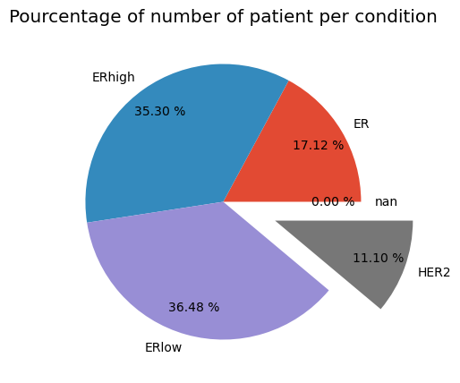
print(f'Number of patient CHEMOTHERAPY Yes :%i'  %metadata[metadata['CHEMOTHERAPY']=='YES'].count()[0])
print(f'Number of patient CHEMOTHERAPY NO :%i'  %metadata[metadata['CHEMOTHERAPY']=='NO'].count()[0])
Number of patient CHEMOTHERAPY Yes :396
Number of patient CHEMOTHERAPY NO :1501
Outcome = pd.DataFrame(metadata['CHEMOTHERAPY'])
Outcome.head()| CHEMOTHERAPY | |
|---|---|
| 0 | NO |
| 1 | NO |
| 2 | YES |
| 3 | YES |
| 4 | YES |
Outcome = Outcome.replace("YES",1)
Outcome = Outcome.replace("NO",0)
Outcome.head()| CHEMOTHERAPY | |
|---|---|
| 0 | 0 |
| 1 | 0 |
| 2 | 1 |
| 3 | 1 |
| 4 | 1 |
print('Labels counts in Outcome Yes and No respectively:', np.bincount(Outcome['CHEMOTHERAPY']))Labels counts in Outcome Yes and No respectively: [1501 396]here we are clearly dealing with class imbalance.
df.index = metadata['PATIENT_ID']
Outcome.index = metadata['PATIENT_ID']
Outcome = Outcome[Outcome.index.isin(df.index)]
Outcome.head()| CHEMOTHERAPY | |
|---|---|
| PATIENT_ID | |
| MB-0000 | 0 |
| MB-0002 | 0 |
| MB-0005 | 1 |
| MB-0006 | 1 |
| MB-0008 | 1 |
Class imbalance correct using imblearn
#!pip install -U imbalanced-learn
from imblearn.over_sampling import RandomOverSampler
ros = RandomOverSampler(random_state=0)
df_resampled, Outcome_resampled = ros.fit_resample(df, Outcome['CHEMOTHERAPY'])from collections import Counter
print(sorted(Counter(Outcome_resampled).items()))[(0, 1501), (1, 1501)]print('Labels counts in Outcome are now:', np.bincount(Outcome_resampled))Labels counts in Outcome are now: [1501 1501]Data preparation for deep learning model
df_resampled = df_resampled.astype('float32')
Outcome_resampled = Outcome_resampled.astype('float32')
X_train, X_test, Y_train, Y_test = train_test_split(df_resampled, Outcome_resampled,
test_size=0.3, random_state=42, shuffle=True)print(f"X_train.shape = {X_train.shape}")
print(f"X_train.dtypes = {X_train.dtypes}")X_train.shape = (2101, 295)
X_train.dtypes = CD52 float32
DARC float32
DCN float32
DB005376 float32
TAT float32
...
CCL5 float32
TFF3 float32
CDH3 float32
SLC39A6 float32
SHISA2 float32
Length: 295, dtype: objectx_train, x_val, y_train, y_val = train_test_split(X_train, Y_train,
shuffle=True)scaler = MinMaxScaler()
x_train_scaled = scaler.fit_transform(x_train)
x_val_scaled = scaler.transform(x_val)
x_test_scaled = scaler.transform(X_test)print(f"x_train_scaled.shape = {x_train_scaled.shape}")
print(f"x_val_scaled.shape = {x_val_scaled.shape}")
print(f"x_test_scaled.shape = {x_test_scaled.shape}")x_train_scaled.shape = (1575, 295)
x_val_scaled.shape = (526, 295)
x_test_scaled.shape = (901, 295)y_train = np.asarray(y_train).astype('float32').reshape((-1,1))
y_trainarray([[1.],
[0.],
[0.],
...,
[1.],
[1.],
[0.]], dtype=float32)Model
EPOCHS = 50
NB_CLASSES = 1
DROPOUT = 0.3
# The model hyperparatmeter was defined with gridSearchCV using scikeras.wrappers, see below at the end of this notebook.
model = Sequential()
model.add(Dense(20, input_shape=x_train_scaled.shape[1:], activation = 'relu', name='dense_layer'))
model.add(Dropout(DROPOUT))
model.add(Dense(10, activation = 'relu', name='dense_layer_2',
kernel_regularizer=regularizers.L1(0.01),
activity_regularizer=regularizers.L2(0.01)))
model.add(Dropout(DROPOUT))
model.add(Dense(NB_CLASSES, activation= "sigmoid", name='dense_layer_4')) model.summary()Model: "sequential_7"
_________________________________________________________________
Layer (type) Output Shape Param #
=================================================================
dense_layer (Dense) (None, 20) 5920
dropout_14 (Dropout) (None, 20) 0
dense_layer_2 (Dense) (None, 10) 210
dropout_15 (Dropout) (None, 10) 0
dense_layer_4 (Dense) (None, 1) 11
=================================================================
Total params: 6141 (23.99 KB)
Trainable params: 6141 (23.99 KB)
Non-trainable params: 0 (0.00 Byte)
_________________________________________________________________keras.utils.plot_model(model, show_shapes=True)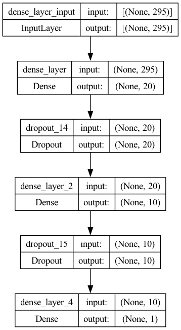
early_stopping = EarlyStopping(
    patience  = 10,     # how many epochs to wait before stopping
    restore_best_weights=True,
)
model.compile(loss="binary_crossentropy", optimizer=tf.keras.optimizers.Adam(), metrics=["accuracy"])WARNING:absl:At this time, the v2.11+ optimizer `tf.keras.optimizers.Adam` runs slowly on M1/M2 Macs, please use the legacy Keras optimizer instead, located at `tf.keras.optimizers.legacy.Adam`.
WARNING:absl:There is a known slowdown when using v2.11+ Keras optimizers on M1/M2 Macs. Falling back to the legacy Keras optimizer, i.e., `tf.keras.optimizers.legacy.Adam`.#training the moodel
results = model.fit(x_train_scaled, y_train, epochs=EPOCHS,
verbose=1, callbacks=[early_stopping],
validation_data=(x_val_scaled, y_val))Epoch 1/50
1/50 [..............................] - ETA: 16s - loss: 1.8349 - accuracy: 0.3438
2024-02-21 13:24:19.384159: I tensorflow/core/grappler/optimizers/custom_graph_optimizer_registry.cc:114] Plugin optimizer for device_type GPU is enabled.
50/50 [==============================] - 1s 15ms/step - loss: 1.3913 - accuracy: 0.5213 - val_loss: 1.0835 - val_accuracy: 0.6939
Epoch 2/50
2024-02-21 13:24:20.105497: I tensorflow/core/grappler/optimizers/custom_graph_optimizer_registry.cc:114] Plugin optimizer for device_type GPU is enabled.
50/50 [==============================] - 1s 11ms/step - loss: 1.2134 - accuracy: 0.6070 - val_loss: 1.0067 - val_accuracy: 0.7281
Epoch 3/50
50/50 [==============================] - 1s 10ms/step - loss: 1.1318 - accuracy: 0.6438 - val_loss: 0.9373 - val_accuracy: 0.7414
Epoch 4/50
50/50 [==============================] - 1s 10ms/step - loss: 1.0318 - accuracy: 0.6838 - val_loss: 0.8786 - val_accuracy: 0.7452
Epoch 5/50
50/50 [==============================] - 1s 10ms/step - loss: 0.9836 - accuracy: 0.6863 - val_loss: 0.8317 - val_accuracy: 0.7548
Epoch 6/50
50/50 [==============================] - 1s 11ms/step - loss: 0.8729 - accuracy: 0.7257 - val_loss: 0.7855 - val_accuracy: 0.7605
Epoch 7/50
50/50 [==============================] - 1s 11ms/step - loss: 0.8293 - accuracy: 0.7149 - val_loss: 0.7438 - val_accuracy: 0.7624
Epoch 8/50
50/50 [==============================] - 1s 10ms/step - loss: 0.7853 - accuracy: 0.7422 - val_loss: 0.7088 - val_accuracy: 0.7624
Epoch 9/50
50/50 [==============================] - 1s 11ms/step - loss: 0.7416 - accuracy: 0.7416 - val_loss: 0.6783 - val_accuracy: 0.7624
Epoch 10/50
50/50 [==============================] - 1s 10ms/step - loss: 0.7064 - accuracy: 0.7460 - val_loss: 0.6627 - val_accuracy: 0.7529
Epoch 11/50
50/50 [==============================] - 1s 10ms/step - loss: 0.6734 - accuracy: 0.7543 - val_loss: 0.6347 - val_accuracy: 0.7643
Epoch 12/50
50/50 [==============================] - 1s 10ms/step - loss: 0.6524 - accuracy: 0.7581 - val_loss: 0.6396 - val_accuracy: 0.7376
Epoch 13/50
50/50 [==============================] - 1s 10ms/step - loss: 0.6322 - accuracy: 0.7606 - val_loss: 0.6078 - val_accuracy: 0.7662
Epoch 14/50
50/50 [==============================] - 1s 10ms/step - loss: 0.6250 - accuracy: 0.7638 - val_loss: 0.5963 - val_accuracy: 0.7852
Epoch 15/50
50/50 [==============================] - 1s 10ms/step - loss: 0.6061 - accuracy: 0.7600 - val_loss: 0.5883 - val_accuracy: 0.7738
Epoch 16/50
50/50 [==============================] - 1s 10ms/step - loss: 0.5981 - accuracy: 0.7790 - val_loss: 0.5958 - val_accuracy: 0.7471
Epoch 17/50
50/50 [==============================] - 1s 10ms/step - loss: 0.5931 - accuracy: 0.7695 - val_loss: 0.5864 - val_accuracy: 0.7529
Epoch 18/50
50/50 [==============================] - 1s 10ms/step - loss: 0.5850 - accuracy: 0.7683 - val_loss: 0.5733 - val_accuracy: 0.7776
Epoch 19/50
50/50 [==============================] - 1s 10ms/step - loss: 0.5831 - accuracy: 0.7708 - val_loss: 0.5731 - val_accuracy: 0.7605
Epoch 20/50
50/50 [==============================] - 1s 10ms/step - loss: 0.5710 - accuracy: 0.7778 - val_loss: 0.5601 - val_accuracy: 0.8004
Epoch 21/50
50/50 [==============================] - 1s 10ms/step - loss: 0.5670 - accuracy: 0.7746 - val_loss: 0.5532 - val_accuracy: 0.7795
Epoch 22/50
50/50 [==============================] - 1s 10ms/step - loss: 0.5594 - accuracy: 0.7854 - val_loss: 0.5508 - val_accuracy: 0.7909
Epoch 23/50
50/50 [==============================] - 1s 10ms/step - loss: 0.5434 - accuracy: 0.7898 - val_loss: 0.5430 - val_accuracy: 0.8023
Epoch 24/50
50/50 [==============================] - 1s 10ms/step - loss: 0.5484 - accuracy: 0.7714 - val_loss: 0.5388 - val_accuracy: 0.7928
Epoch 25/50
50/50 [==============================] - 1s 10ms/step - loss: 0.5373 - accuracy: 0.7835 - val_loss: 0.5358 - val_accuracy: 0.7909
Epoch 26/50
50/50 [==============================] - 1s 10ms/step - loss: 0.5299 - accuracy: 0.7867 - val_loss: 0.5334 - val_accuracy: 0.7985
Epoch 27/50
50/50 [==============================] - 1s 10ms/step - loss: 0.5288 - accuracy: 0.8006 - val_loss: 0.5296 - val_accuracy: 0.8004
Epoch 28/50
50/50 [==============================] - 1s 11ms/step - loss: 0.5275 - accuracy: 0.8038 - val_loss: 0.5288 - val_accuracy: 0.8042
Epoch 29/50
50/50 [==============================] - 1s 11ms/step - loss: 0.5140 - accuracy: 0.8070 - val_loss: 0.5283 - val_accuracy: 0.7985
Epoch 30/50
50/50 [==============================] - 1s 10ms/step - loss: 0.5121 - accuracy: 0.8083 - val_loss: 0.5249 - val_accuracy: 0.8061
Epoch 31/50
50/50 [==============================] - 1s 11ms/step - loss: 0.5249 - accuracy: 0.7873 - val_loss: 0.5189 - val_accuracy: 0.8080
Epoch 32/50
50/50 [==============================] - 1s 11ms/step - loss: 0.5142 - accuracy: 0.8063 - val_loss: 0.5157 - val_accuracy: 0.8118
Epoch 33/50
50/50 [==============================] - 1s 10ms/step - loss: 0.4996 - accuracy: 0.8140 - val_loss: 0.5171 - val_accuracy: 0.8156
Epoch 34/50
50/50 [==============================] - 1s 11ms/step - loss: 0.5088 - accuracy: 0.8038 - val_loss: 0.5152 - val_accuracy: 0.8137
Epoch 35/50
50/50 [==============================] - 1s 11ms/step - loss: 0.5053 - accuracy: 0.8076 - val_loss: 0.5087 - val_accuracy: 0.8194
Epoch 36/50
50/50 [==============================] - 1s 11ms/step - loss: 0.4938 - accuracy: 0.8159 - val_loss: 0.5094 - val_accuracy: 0.8137
Epoch 37/50
50/50 [==============================] - 1s 12ms/step - loss: 0.4895 - accuracy: 0.8159 - val_loss: 0.5018 - val_accuracy: 0.8194
Epoch 38/50
50/50 [==============================] - 1s 12ms/step - loss: 0.4831 - accuracy: 0.8184 - val_loss: 0.5098 - val_accuracy: 0.8080
Epoch 39/50
50/50 [==============================] - 1s 10ms/step - loss: 0.4847 - accuracy: 0.8248 - val_loss: 0.5049 - val_accuracy: 0.8270
Epoch 40/50
50/50 [==============================] - 1s 10ms/step - loss: 0.4944 - accuracy: 0.8165 - val_loss: 0.4978 - val_accuracy: 0.8194
Epoch 41/50
50/50 [==============================] - 1s 11ms/step - loss: 0.4819 - accuracy: 0.8260 - val_loss: 0.4957 - val_accuracy: 0.8137
Epoch 42/50
50/50 [==============================] - 1s 11ms/step - loss: 0.4716 - accuracy: 0.8140 - val_loss: 0.4952 - val_accuracy: 0.8213
Epoch 43/50
50/50 [==============================] - 1s 10ms/step - loss: 0.4745 - accuracy: 0.8317 - val_loss: 0.4968 - val_accuracy: 0.8156
Epoch 44/50
50/50 [==============================] - 1s 10ms/step - loss: 0.4653 - accuracy: 0.8356 - val_loss: 0.4997 - val_accuracy: 0.8175
Epoch 45/50
50/50 [==============================] - 1s 10ms/step - loss: 0.4777 - accuracy: 0.8324 - val_loss: 0.4920 - val_accuracy: 0.8156
Epoch 46/50
50/50 [==============================] - 1s 10ms/step - loss: 0.4689 - accuracy: 0.8279 - val_loss: 0.4885 - val_accuracy: 0.8194
Epoch 47/50
50/50 [==============================] - 1s 10ms/step - loss: 0.4715 - accuracy: 0.8190 - val_loss: 0.5085 - val_accuracy: 0.8023
Epoch 48/50
50/50 [==============================] - 1s 11ms/step - loss: 0.4647 - accuracy: 0.8286 - val_loss: 0.4928 - val_accuracy: 0.8137
Epoch 49/50
50/50 [==============================] - 1s 10ms/step - loss: 0.4521 - accuracy: 0.8400 - val_loss: 0.4929 - val_accuracy: 0.8137
Epoch 50/50
50/50 [==============================] - 1s 10ms/step - loss: 0.4719 - accuracy: 0.8254 - val_loss: 0.4839 - val_accuracy: 0.8232pd.DataFrame(results.history).plot(figsize=(8, 5))
plt.grid(True)
plt.gca().set_ylim(0, 1)
plt.show()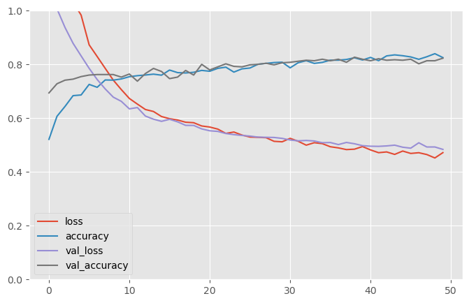
#evalute the model
test_loss, test_acc = model.evaluate(x_test_scaled, Y_test)
print('Test accuracy:', test_acc)
29/29 [==============================] - 0s 10ms/step - loss: 0.4760 - accuracy: 0.8113
Test accuracy: 0.8113207817077637# making prediction
predictions = model.predict(X_test)29/29 [==============================] - 0s 2ms/step
2024-02-21 13:24:46.547168: I tensorflow/core/grappler/optimizers/custom_graph_optimizer_registry.cc:114] Plugin optimizer for device_type GPU is enabled.predicted = tf.squeeze(predictions)
predicted = np.array([1 if x >= 0.5 else 0 for x in predicted])
actual = np.array(Y_test)
conf_mat = confusion_matrix(actual, predicted)
displ = ConfusionMatrixDisplay(confusion_matrix=conf_mat)
displ.plot()<sklearn.metrics._plot.confusion_matrix.ConfusionMatrixDisplay at 0x3363f3580>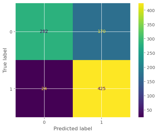
Explainability
Explain tensorflow keras model with shap DeepExplainer
sample_size=500
if sample_size>len(X_train.values):
  sample_size=len(X_train.values)

explainer = shap.DeepExplainer(model, X_train.values[:sample_size], y_train)
Your TensorFlow version is newer than 2.4.0 and so graph support has been removed in eager mode and some static graphs may not be supported. See PR #1483 for discussion.# Explain the SHAP values for the whole dataset
# to test the SHAP explainer.
shap_values = explainer.shap_values(X_train.values[:sample_size], ranked_outputs=None)`tf.keras.backend.set_learning_phase` is deprecated and will be removed after 2020-10-11. To update it, simply pass a True/False value to the `training` argument of the `__call__` method of your layer or model.
2024-02-21 13:26:40.355386: I tensorflow/core/grappler/optimizers/custom_graph_optimizer_registry.cc:114] Plugin optimizer for device_type GPU is enabled.shap_values[array([[-6.13931217e-04, 5.79104235e-04, 1.21821380e-04, ...,
3.32532691e-05, 5.89004019e-04, 2.54693348e-03],
[ 1.22798362e-03, 1.75002951e-03, -6.65651402e-04, ...,
9.90149798e-04, 1.52458099e-03, 1.27402262e-03],
[ 2.40881299e-03, -6.52628345e-03, 9.89748398e-04, ...,
-9.38840210e-04, -2.61786184e-03, -5.97110670e-03],
...,
[ 4.05412196e-04, 1.70486758e-03, -2.36380190e-04, ...,
3.85903375e-04, -2.11221166e-03, 2.30341917e-03],
[ 7.42328644e-04, 7.09563727e-04, 1.07669597e-03, ...,
-4.93239932e-05, 9.01810999e-04, -3.41807390e-05],
[-1.20005244e-03, 1.12299132e-03, -7.52978318e-04, ...,
2.85379556e-05, 7.02320656e-04, 9.09106282e-04]])]print(" The shap values length is egal to the number of the model's output:", len(shap_values)) The shap values length is egal to the number of the model's output: 1# #shap_values
# shap.initjs()
# shap.force_plot(explainer.expected_value[0].numpy(), shap_values[0], X_train, link="logit")def get_fetaure_importnace(shap_values, features, num=0):
"Features is the X_train.columns names"
vals = np.abs(pd.DataFrame(shap_values[num]).values).mean(0)
shap_importance = pd.DataFrame(list(zip(features, vals)), columns=['col_name', 'feature_importance_vals'])
shap_importance.sort_values(by=['feature_importance_vals'], ascending=False, inplace=True)
shap_importance.loc[shap_importance['feature_importance_vals']>0]
return shap_importanceshap_importance = get_fetaure_importnace(shap_values, features=X_train.columns, num=0)
shap_importance| col_name | feature_importance_vals | |
|---|---|---|
| 131 | ESR1 | 0.010920 |
| 279 | FOSB | 0.007193 |
| 280 | CLEC3A | 0.006748 |
| 245 | BEX1 | 0.006334 |
| 110 | IGJ | 0.005912 |
| ... | ... | ... |
| 156 | RPL14 | 0.000166 |
| 212 | PRODH | 0.000164 |
| 125 | TGFBR3 | 0.000143 |
| 220 | IRX2 | 0.000127 |
| 158 | CD79A | 0.000042 |
295 rows × 2 columns
def plot_importance_features(Features, top=10, title=" "):

    " Features are a 2 colunms dataframe with features names and weights"

    fig, ax = plt.subplots(figsize =(5, 5))
    top_features = Features.iloc[:top]
    # Horizontal Bar Plot
    ax.barh(top_features['col_name'], top_features['feature_importance_vals'])
    ax.set_yticks(top_features['col_name'])
    ax.invert_yaxis()  # labels read top-to-bottom
    ax.set_xlabel('Importance')
    ax.set_title(title)
    plot = plt.show()
    return plot
plot_importance_features(Features=shap_importance, top=10, title="Shap importance features")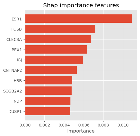
# visualize the first prediction's explanation (use matplotlib=True to avoid Javascript)
shap.summary_plot(shap_values[0], X_test, plot_type="bar", max_display=10)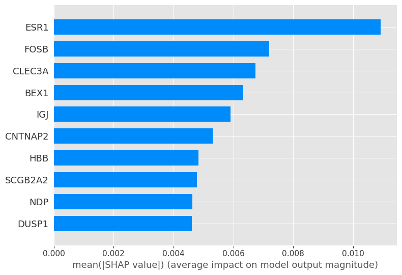
shap.summary_plot(shap_values[0], features=X_train.values[:sample_size], feature_names=X_train.columns, show=False, plot_type="dot", max_display=10)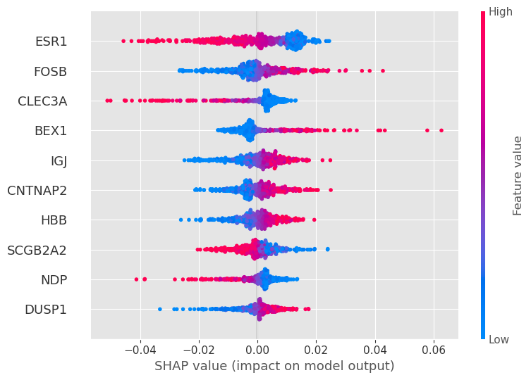
Explain tensorflow keras model with weights
def get_weights_importnace(model, features, num=0):
    "Features are the  X_train.columns names"
    vals_weights = np.abs(model.layers[num].get_weights()[0].T).mean(0)
    weights_importance = pd.DataFrame(list(zip(features, vals_weights)), columns=['col_name', 'feature_importance_vals'])
    weights_importance.sort_values(by=['feature_importance_vals'], ascending=False, inplace=True)
    weights_importance.loc[weights_importance['feature_importance_vals']>0]
    return weights_importance
weights_importance = get_weights_importnace(model, features= X_train.columns)
weights_importance| col_name | feature_importance_vals | |
|---|---|---|
| 131 | ESR1 | 0.156979 |
| 228 | GRIA2 | 0.142732 |
| 271 | FABP7 | 0.133380 |
| 124 | NTN4 | 0.129271 |
| 70 | HOXB5 | 0.127729 |
| ... | ... | ... |
| 146 | KRT7 | 0.049167 |
| 115 | MFAP4 | 0.048581 |
| 34 | C19orf33 | 0.046389 |
| 208 | TPSAB1 | 0.046116 |
| 174 | ZG16B | 0.043745 |
295 rows × 2 columns
plot_importance_features(Features=weights_importance, top=10, title="Weights importance features")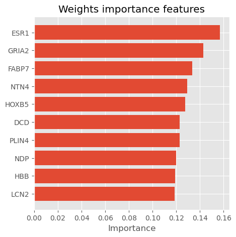
Hyperparameter tunning with GridSearchCV using scikeras.wrappers
def get_model(nb_hidden, nb_neurons):
    print(f"##  {nb_hidden}-{nb_neurons}   ##")
    model = keras.models.Sequential()
    model.add(Dense(64, input_shape=x_train_scaled.shape[1:], activation = 'relu', name='dense_layer'))
    model.add(keras.layers.Dense(2 * nb_neurons, activation="relu"))
    if nb_hidden > 1 :
        for layer in range(2, nb_hidden):
            model.add(keras.layers.Dense(nb_neurons, activation="relu"))
    model.add(keras.layers.Dense(1, activation="sigmoid" ))

    model.compile(loss="binary_crossentropy", optimizer="adam", metrics=["accuracy"])

    return model
#!pip install scikeras
from scikeras.wrappers import KerasClassifier
keras_classifier = KerasClassifier(get_model, nb_hidden=1, nb_neurons=1)
param_distribs = {
"nb_hidden": [1,2,3,6,8],
"nb_neurons": [3,5,8,10],
}
early_stopping = keras.callbacks.EarlyStopping(patience=10, restore_best_weights=True)
search_cv = GridSearchCV(keras_classifier, param_distribs, cv=2 )
search_cv.fit(x_train_scaled, y_train, epochs=20, callbacks=[early_stopping], validation_data=[x_val_scaled, y_val], )
print(f"search_cv.best_params_ = {search_cv.best_params_}")

print(f"search_cv.best_score_ = {search_cv.best_score_}") print(f"search_cv.best_params_ = {search_cv.best_params_}")
print(f"search_cv.best_score_ = {search_cv.best_score_}") search_cv.best_params_ = {'nb_hidden': 1, 'nb_neurons': 10}
search_cv.best_score_ = 0.810161475499713