SHAP and LIME on MOLECULAR TAXONOMY OF BREAST CANCER INTERNATIONAL CONSORTIUM (METABRIC)
import pandas as pd
import numpy as np
import matplotlib.pyplot as plt
import plotly.express as px
import seaborn as sns
import session_info
import xgboost as xgb
import random
from lime import lime_tabular
from sklearn.model_selection import train_test_split, StratifiedKFold
import lime
import shap
import warnings
warnings.filterwarnings('ignore')
Data load and preprocessing
Expression data
df = pd.read_csv("/Users/lamine/Explainqble AI /metabric_test.csv")
df.head(5)| CD52 | DARC | DCN | DB005376 | TAT | GSTM1 | UGT2B11 | AKR7A3 | SERHL2 | ASS1 | ... | MYB | PROM1 | GSTT1 | NELL2 | CST5 | CCL5 | TFF3 | CDH3 | SLC39A6 | SHISA2 | |
|---|---|---|---|---|---|---|---|---|---|---|---|---|---|---|---|---|---|---|---|---|---|
| 0 | 8.240128 | 10.731211 | 11.251592 | 5.350604 | 5.698745 | 5.626606 | 5.845062 | 8.334491 | 7.150713 | 9.887783 | ... | 7.864506 | 10.475799 | 5.236212 | 6.462909 | 5.333817 | 8.771015 | 10.545305 | 8.588759 | 8.287300 | 6.155340 |
| 1 | 7.441887 | 6.498731 | 9.968656 | 5.701508 | 5.416231 | 5.108180 | 5.382890 | 10.277779 | 6.070879 | 6.203103 | ... | 10.699097 | 5.977531 | 8.450049 | 7.486917 | 5.464502 | 8.216436 | 10.422146 | 5.838056 | 10.380559 | 9.409817 |
| 2 | 7.977708 | 6.615727 | 9.632207 | 6.346358 | 5.480066 | 5.356168 | 7.798285 | 9.117568 | 6.230590 | 7.928613 | ... | 9.861437 | 8.517411 | 7.230715 | 11.957439 | 5.359362 | 8.012079 | 12.201802 | 6.681570 | 10.009376 | 9.094121 |
| 3 | 8.045781 | 5.806614 | 8.927632 | 5.628718 | 5.746114 | 5.402901 | 6.043053 | 10.057702 | 11.682904 | 10.047193 | ... | 9.138474 | 9.099391 | 8.072639 | 12.478907 | 5.523048 | 9.245577 | 14.169804 | 6.392376 | 11.141299 | 10.039994 |
| 4 | 9.001653 | 7.928994 | 9.356798 | 5.484226 | 5.152513 | 5.401268 | 8.511554 | 11.127156 | 7.472530 | 7.200276 | ... | 9.591358 | 7.264378 | 8.975517 | 10.044922 | 5.034380 | 10.243518 | 13.568835 | 8.476834 | 8.916101 | 5.929184 |
5 rows × 295 columns
df.info()<class 'pandas.core.frame.DataFrame'>
RangeIndex: 1897 entries, 0 to 1896
Columns: 295 entries, CD52 to SHISA2
dtypes: float64(295)
memory usage: 4.3 MBdf.describe()| CD52 | DARC | DCN | DB005376 | TAT | GSTM1 | UGT2B11 | AKR7A3 | SERHL2 | ASS1 | ... | MYB | PROM1 | GSTT1 | NELL2 | CST5 | CCL5 | TFF3 | CDH3 | SLC39A6 | SHISA2 | |
|---|---|---|---|---|---|---|---|---|---|---|---|---|---|---|---|---|---|---|---|---|---|
| count | 1897.000000 | 1897.000000 | 1897.000000 | 1897.000000 | 1897.000000 | 1897.000000 | 1897.000000 | 1897.000000 | 1897.000000 | 1897.000000 | ... | 1897.000000 | 1897.000000 | 1897.000000 | 1897.000000 | 1897.000000 | 1897.000000 | 1897.000000 | 1897.000000 | 1897.000000 | 1897.000000 |
| mean | 8.522002 | 7.439279 | 8.592254 | 6.084079 | 6.267616 | 6.477882 | 6.920908 | 9.397352 | 7.558455 | 8.298495 | ... | 9.743111 | 8.041666 | 8.295523 | 7.466347 | 6.033271 | 9.845330 | 11.742209 | 7.465389 | 9.204424 | 7.725656 |
| std | 1.349624 | 1.323882 | 1.366120 | 1.489150 | 1.623607 | 1.490238 | 2.132190 | 1.280389 | 1.724598 | 1.314099 | ... | 1.242550 | 1.996117 | 1.691650 | 1.532031 | 1.500256 | 1.357065 | 2.444823 | 1.274105 | 1.620264 | 1.659966 |
| min | 5.018810 | 5.099984 | 5.074217 | 4.922326 | 4.925973 | 4.939510 | 4.988302 | 6.888636 | 5.214098 | 5.001618 | ... | 5.565536 | 5.047322 | 4.854543 | 5.030010 | 4.965204 | 5.685101 | 5.154748 | 5.103031 | 5.510203 | 5.119337 |
| 25% | 7.526147 | 6.337077 | 7.585572 | 5.315275 | 5.400663 | 5.428807 | 5.547688 | 8.359180 | 6.265815 | 7.277712 | ... | 9.072006 | 6.297426 | 7.469392 | 6.264153 | 5.337878 | 8.875585 | 10.657896 | 6.461509 | 7.869267 | 6.363869 |
| 50% | 8.448275 | 7.331663 | 8.608817 | 5.461374 | 5.563156 | 5.624529 | 5.881415 | 9.331409 | 7.083379 | 8.280220 | ... | 10.023695 | 7.623121 | 8.889979 | 7.056264 | 5.484401 | 9.857851 | 12.473404 | 7.303850 | 9.201048 | 7.358426 |
| 75% | 9.428863 | 8.370030 | 9.566763 | 5.971988 | 6.175448 | 7.490048 | 7.556015 | 10.241203 | 8.371308 | 9.256413 | ... | 10.654395 | 9.607842 | 9.489065 | 8.371956 | 5.818663 | 10.791775 | 13.588736 | 8.255375 | 10.508201 | 8.869039 |
| max | 13.374739 | 11.619202 | 12.478475 | 13.010996 | 13.166804 | 12.070735 | 14.145451 | 13.512971 | 13.731721 | 12.182876 | ... | 12.091906 | 13.569006 | 12.784519 | 13.110442 | 13.922840 | 14.004198 | 14.808641 | 12.003642 | 13.440167 | 12.874823 |
8 rows × 295 columns
label data
metadata = pd.read_csv("/Users/lamine/Explainqble AI /metabric_clin.csv")
metadata.head(5)| PATIENT_ID | LYMPH_NODES_EXAMINED_POSITIVE | NPI | CELLULARITY | CHEMOTHERAPY | COHORT | ER_IHC | HER2_SNP6 | HORMONE_THERAPY | INFERRED_MENOPAUSAL_STATE | ... | OS_STATUS | CLAUDIN_SUBTYPE | THREEGENE | VITAL_STATUS | LATERALITY | RADIO_THERAPY | HISTOLOGICAL_SUBTYPE | BREAST_SURGERY | RFS_STATUS | RFS_MONTHS | |
|---|---|---|---|---|---|---|---|---|---|---|---|---|---|---|---|---|---|---|---|---|---|
| 0 | MB-0000 | 10.0 | 6.044 | NaN | NO | 1.0 | Positve | NEUTRAL | YES | Post | ... | 0:LIVING | claudin-low | ER-/HER2- | Living | Right | YES | Ductal/NST | MASTECTOMY | 0:Not Recurred | 138.65 |
| 1 | MB-0002 | 0.0 | 4.020 | High | NO | 1.0 | Positve | NEUTRAL | YES | Pre | ... | 0:LIVING | LumA | ER+/HER2- High Prolif | Living | Right | YES | Ductal/NST | BREAST CONSERVING | 0:Not Recurred | 83.52 |
| 2 | MB-0005 | 1.0 | 4.030 | High | YES | 1.0 | Positve | NEUTRAL | YES | Pre | ... | 1:DECEASED | LumB | NaN | Died of Disease | Right | NO | Ductal/NST | MASTECTOMY | 1:Recurred | 151.28 |
| 3 | MB-0006 | 3.0 | 4.050 | Moderate | YES | 1.0 | Positve | NEUTRAL | YES | Pre | ... | 0:LIVING | LumB | NaN | Living | Right | YES | Mixed | MASTECTOMY | 0:Not Recurred | 162.76 |
| 4 | MB-0008 | 8.0 | 6.080 | High | YES | 1.0 | Positve | NEUTRAL | YES | Post | ... | 1:DECEASED | LumB | ER+/HER2- High Prolif | Died of Disease | Right | YES | Mixed | MASTECTOMY | 1:Recurred | 18.55 |
5 rows × 24 columns
metadata.info()<class 'pandas.core.frame.DataFrame'>
RangeIndex: 1897 entries, 0 to 1896
Data columns (total 24 columns):
# Column Non-Null Count Dtype
--- ------ -------------- -----
0 PATIENT_ID 1897 non-null object
1 LYMPH_NODES_EXAMINED_POSITIVE 1897 non-null float64
2 NPI 1897 non-null float64
3 CELLULARITY 1843 non-null object
4 CHEMOTHERAPY 1897 non-null object
5 COHORT 1897 non-null float64
6 ER_IHC 1867 non-null object
7 HER2_SNP6 1897 non-null object
8 HORMONE_THERAPY 1897 non-null object
9 INFERRED_MENOPAUSAL_STATE 1897 non-null object
10 SEX 1897 non-null object
11 INTCLUST 1897 non-null object
12 AGE_AT_DIAGNOSIS 1897 non-null float64
13 OS_MONTHS 1897 non-null float64
14 OS_STATUS 1897 non-null object
15 CLAUDIN_SUBTYPE 1897 non-null object
16 THREEGENE 1694 non-null object
17 VITAL_STATUS 1897 non-null object
18 LATERALITY 1792 non-null object
19 RADIO_THERAPY 1897 non-null object
20 HISTOLOGICAL_SUBTYPE 1882 non-null object
21 BREAST_SURGERY 1875 non-null object
22 RFS_STATUS 1897 non-null object
23 RFS_MONTHS 1897 non-null float64
dtypes: float64(6), object(18)
memory usage: 355.8+ KBmetadata.columnsIndex(['PATIENT_ID', 'LYMPH_NODES_EXAMINED_POSITIVE', 'NPI', 'CELLULARITY',
'CHEMOTHERAPY', 'COHORT', 'ER_IHC', 'HER2_SNP6', 'HORMONE_THERAPY',
'INFERRED_MENOPAUSAL_STATE', 'SEX', 'INTCLUST', 'AGE_AT_DIAGNOSIS',
'OS_MONTHS', 'OS_STATUS', 'CLAUDIN_SUBTYPE', 'THREEGENE',
'VITAL_STATUS', 'LATERALITY', 'RADIO_THERAPY', 'HISTOLOGICAL_SUBTYPE',
'BREAST_SURGERY', 'RFS_STATUS', 'RFS_MONTHS'],
dtype='object')print(f"The total patient ids are {metadata['PATIENT_ID'].count()}, from those the unique ids are {metadata['PATIENT_ID'].value_counts().shape[0]} ")The total patient ids are 1897, from those the unique ids are 1897columns = metadata.keys()
columns = list(columns)
print(columns)['PATIENT_ID', 'LYMPH_NODES_EXAMINED_POSITIVE', 'NPI', 'CELLULARITY', 'CHEMOTHERAPY', 'COHORT', 'ER_IHC', 'HER2_SNP6', 'HORMONE_THERAPY', 'INFERRED_MENOPAUSAL_STATE', 'SEX', 'INTCLUST', 'AGE_AT_DIAGNOSIS', 'OS_MONTHS', 'OS_STATUS', 'CLAUDIN_SUBTYPE', 'THREEGENE', 'VITAL_STATUS', 'LATERALITY', 'RADIO_THERAPY', 'HISTOLOGICAL_SUBTYPE', 'BREAST_SURGERY', 'RFS_STATUS', 'RFS_MONTHS']# Remove unnecesary elements
columns.remove('PATIENT_ID')
# Get the total classes
print(f"There are {len(columns)} columns of labels for these conditions: {columns}")There are 23 columns of labels for these conditions: ['LYMPH_NODES_EXAMINED_POSITIVE', 'NPI', 'CELLULARITY', 'CHEMOTHERAPY', 'COHORT', 'ER_IHC', 'HER2_SNP6', 'HORMONE_THERAPY', 'INFERRED_MENOPAUSAL_STATE', 'SEX', 'INTCLUST', 'AGE_AT_DIAGNOSIS', 'OS_MONTHS', 'OS_STATUS', 'CLAUDIN_SUBTYPE', 'THREEGENE', 'VITAL_STATUS', 'LATERALITY', 'RADIO_THERAPY', 'HISTOLOGICAL_SUBTYPE', 'BREAST_SURGERY', 'RFS_STATUS', 'RFS_MONTHS']metadata['THREEGENE'].unique()array(['ER-/HER2-', 'ER+/HER2- High Prolif', nan, 'ER+/HER2- Low Prolif',
'HER2+'], dtype=object)print(f"The total patient ids are {metadata['PATIENT_ID'].count()}, from those the unique ids CHEMOTHERAPY are {metadata['CHEMOTHERAPY'].value_counts().shape[0]} ")The total patient ids are 1897, from those the unique ids CHEMOTHERAPY are 2print(f'Number of patient ER-/HER2- :%i' %metadata[metadata['THREEGENE']=='ER-/HER2-'].count()[0])
print(f'Number of patient ER+/HER2- High Prolif :%i' %metadata[metadata['THREEGENE']=='ER+/HER2- High Prolif'].count()[0])
print(f'Number of patient ER+/HER2- Low Prolif :%i' %metadata[metadata['THREEGENE']=='ER+/HER2- Low Prolif'].count()[0])
print(f'Number of patient HER2+ :%i' %metadata[metadata['THREEGENE']=='HER2+'].count()[0])
print(f'Number of patient nan :%i' %metadata[metadata['THREEGENE']=='nan'].count()[0])Number of patient ER-/HER2- :290
Number of patient ER+/HER2- High Prolif :598
Number of patient ER+/HER2- Low Prolif :618
Number of patient HER2+ :188
Number of patient nan :0plt.figure(figsize=(8,5), dpi=100)
plt.style.use('ggplot')
ER = metadata[metadata['THREEGENE']=='ER-/HER2-'].count()[0]
ERhigh = metadata[metadata['THREEGENE']=='ER+/HER2- High Prolif'].count()[0]
ERlow = metadata[metadata['THREEGENE']=='ER+/HER2- Low Prolif'].count()[0]
HER2 = metadata[metadata['THREEGENE']=='HER2+'].count()[0]
nan = metadata[metadata['THREEGENE']=='nan'].count()[0]
Condition = [ER, ERhigh, ERlow, HER2, nan]
label = ['ER', 'ERhigh', 'ERlow', 'HER2', 'nan']
explode = (0,0,0,.4,0)
plt.title('Pourcentage of number of patient per condition')
plt.pie(Condition, labels=label, explode=explode, pctdistance=0.8,autopct='%.2f %%')
plt.show()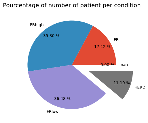
print(f'Number of patient CHEMOTHERAPY Yes :%i'  %metadata[metadata['CHEMOTHERAPY']=='YES'].count()[0])
print(f'Number of patient CHEMOTHERAPY NO :%i'  %metadata[metadata['CHEMOTHERAPY']=='NO'].count()[0])
Number of patient CHEMOTHERAPY Yes :396
Number of patient CHEMOTHERAPY NO :1501
Outcome = pd.DataFrame(metadata['CHEMOTHERAPY'])
Outcome.head()| CHEMOTHERAPY | |
|---|---|
| 0 | NO |
| 1 | NO |
| 2 | YES |
| 3 | YES |
| 4 | YES |
Outcome = Outcome.replace("YES",1)
Outcome = Outcome.replace("NO",0)
Outcome.head()| CHEMOTHERAPY | |
|---|---|
| 0 | 0 |
| 1 | 0 |
| 2 | 1 |
| 3 | 1 |
| 4 | 1 |
print('Labels counts in Outcome Yes and No respectively:', np.bincount(Outcome['CHEMOTHERAPY']))Labels counts in Outcome Yes and No respectively: [1501 396]here we clearly dealing with class imbalance.
df.index = metadata['PATIENT_ID']
Outcome.index = metadata['PATIENT_ID']
Outcome = Outcome[Outcome.index.isin(df.index)]
Outcome.head()here we clearly dealing with class imbalance.
Class imbalance correct using imblearn
#!pip install -U imbalanced-learn
from imblearn.over_sampling import RandomOverSampler
ros = RandomOverSampler(random_state=0)
df_resampled, Outcome_resampled = ros.fit_resample(df, Outcome['CHEMOTHERAPY'])from collections import Counter
print(sorted(Counter(Outcome_resampled).items()))[(0, 1501), (1, 1501)]print('Labels counts in Outcome are now:', np.bincount(Outcome_resampled))Labels counts in Outcome are now: [1501 1501]Model
X_train, X_test, y_train, y_test = train_test_split(df_resampled, Outcome_resampled, test_size=0.3, random_state=42)

model = xgb.XGBClassifier(objective ='binary:logistic', colsample_bytree = 0.3, learning_rate = 0.1,
                max_depth = 5, alpha = 10, n_estimators = 10)
model.fit(X_train, y_train)
pred= model.predict(X_test)
acc = model.score(X_train, y_train)
print(f'Test accuracy: {acc:.3f}')Test accuracy: 0.873y_pred = pd.DataFrame(model.predict(X_test), columns=['pred'], index=X_test.index)
y_pred.head()| pred | |
|---|---|
| 2786 | 1 |
| 2148 | 1 |
| 1410 | 0 |
| 251 | 1 |
| 2506 | 1 |
xgb.plot_importance(model, max_num_features=10)<Axes: title={'center': 'Feature importance'}, xlabel='F score', ylabel='Features'>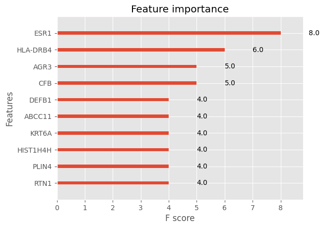
# Using k-fold cross validation to assess model performance
kfold = StratifiedKFold(n_splits=10).split(X_train, y_train)
model = xgb.XGBClassifier(objective ='binary:logistic', colsample_bytree = 0.3, learning_rate = 0.1,
                max_depth = 5, alpha = 10, n_estimators = 10)
scores = []
all_imp = []
for k, (train, test) in enumerate(kfold):
    model.fit(X_train, y_train)
    score = model.score(X_train, y_train)
    scores.append(score)

    print(f'Fold: {k+1:02d}, '
          f'Class distr.: {np.bincount(y_train)}, '
          f'Acc.: {score:.3f}')

mean_acc = np.mean(scores)
std_acc = np.std(scores)
print(f'\nCV accuracy: {mean_acc:.3f} +/- {std_acc:.3f}')
Fold: 01, Class distr.: [1201 1200], Acc.: 0.875
Fold: 02, Class distr.: [1201 1200], Acc.: 0.875
Fold: 03, Class distr.: [1201 1200], Acc.: 0.875
Fold: 04, Class distr.: [1201 1200], Acc.: 0.875
Fold: 05, Class distr.: [1201 1200], Acc.: 0.875
Fold: 06, Class distr.: [1201 1200], Acc.: 0.875
Fold: 07, Class distr.: [1201 1200], Acc.: 0.875
Fold: 08, Class distr.: [1201 1200], Acc.: 0.875
Fold: 09, Class distr.: [1201 1200], Acc.: 0.875
Fold: 10, Class distr.: [1201 1200], Acc.: 0.875
CV accuracy: 0.875 +/- 0.000Explainability
Lime
explainer = lime_tabular.LimeTabularExplainer(
    training_data=np.array(X_train),
    feature_names=X_train.columns,
    class_names= ['NO', 'YES'],
    mode='classification'
)
random.seed(10)
# Choose the instance and use it to predict the results. Here I use the 30th (below the 334 patient).
exp = explainer.explain_instance(
data_row=X_test.iloc[8],
#num_features: maximum number of features present in explanation. I keept default 10.
#num_samples: size of the neighborhood to learn the linear model.Default 500.
predict_fn=model.predict_proba
)
exp.show_in_notebook(show_table=True)# Show the results as list.
exp.as_list()[('9.67 < AGR3 <= 10.83', -0.04316021384209577),
('9.59 < ESR1 <= 10.91', -0.0404119491280816),
('DUSP1 > 11.03', 0.020701450435173546),
('9.45 < GATA3 <= 10.35', -0.015545603987935844),
('CACNA1H <= 6.06', 0.015490266376913983),
('KRT6A <= 5.40', -0.013549350998172813),
('9.35 < TBC1D9 <= 10.32', -0.012658607702864103),
('CALML5 <= 5.89', -0.01245270304063268),
('HOXB5 > 7.31', -0.012228074031454953),
('C1orf106 <= 5.96', -0.009504106297160793)]%matplotlib inline
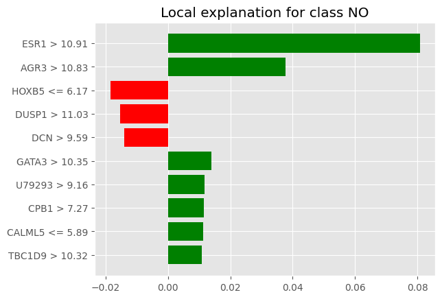
fig = exp.as_pyplot_figure()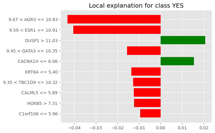
from lime import submodular_pick# Let's use SP-LIME to return explanations on a few sample data sets
# and obtain a non-redundant global decision perspective of the black-box model
sp_exp = submodular_pick.SubmodularPick(explainer,
np.array(X_test),
model.predict_proba,
num_features=10,
num_exps_desired=2) [exp.as_pyplot_figure(label=exp.available_labels()[0]) for exp in sp_exp.sp_explanations]
print('SP-LIME Local Explanations')SP-LIME Local Explanations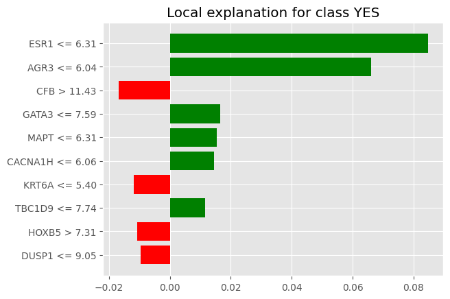
Shap
explainer=shap.Explainer(model)
shap_values = explainer(X_train)
shap_contrib = explainer.shap_values(X_test)
#import Javascript
#shap_values
# This take to much in memory so I am not displaying it.
# shap.initjs(),
# shap.plots.force(shap_values)shap.plots.waterfall(shap_values[0])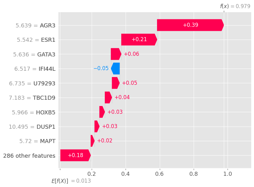
# Global bar plot
shap.plots.bar(shap_values, max_display=8)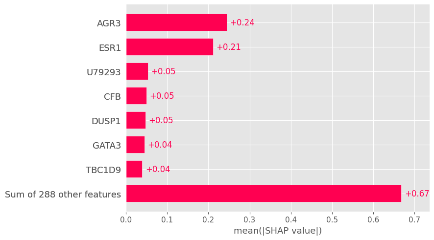
# Local bar plot for the patient 334 (index 8).
shap.plots.bar(shap_values[8], max_display=8)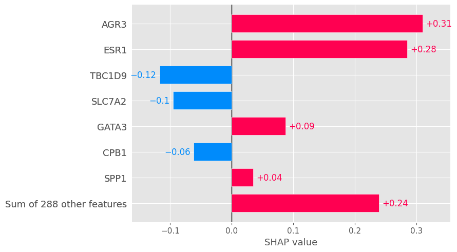
shap.plots.beeswarm(shap_values, max_display=8)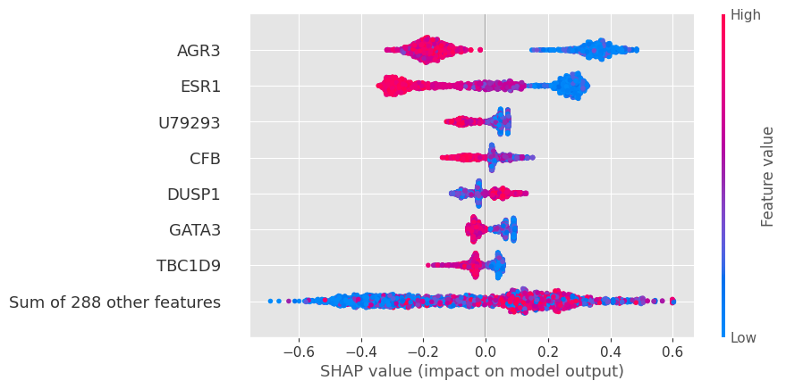
Explainability Tools
Shapash
response_dict = {0: 'NO', 1:'YES'}#!pip install shapash
#
from shapash import SmartExplainer
import tkinter as TK


xpl = SmartExplainer(
    model=model,
    #backend='shap' is the default.
    label_dict=response_dict  #Dictionary mapping integer labels to domain names (classification - target values).
    #preprocessing=encoder,   # Optional: compile step can use inverse_transform method
    #features_dict=name # optional parameter, specifies label for features name
)

xpl.compile(
   contributions=shap_contrib, # Shap Contributions pd.DataFrame
    y_pred=y_pred,  #Prediction values (1 column only)
    x=X_test,  # a preprocessed dataset: Shapash can apply the model to it
    y_target=y_test #Target values (1 column only).
)
xpl.plot.features_importance(max_features=10, label=1)
xpl.plot.scatter_plot_prediction()
#y_pred
xpl.filter(max_contrib=10)
xpl.plot.local_plot(index=334, label='YES')
xpl.plot.compare_plot(row_num=[0, 1, 2, 3, 4, 5, 6], max_features=8)
#Start WebApp
app = xpl.run_app(port=8850, title_story='Explanation')
# Kill the wepapp
app.kill()INFO:root:Your Shapash application run on http://MBP-de-Lamine:8850/
INFO:root:Use the method .kill() to down your app.Explainerdashboard
#!pip install explainerdashboardfrom IPython.core.interactiveshell import InteractiveShell
InteractiveShell.ast_node_interactivity = "all"
from explainerdashboard import ClassifierExplainer, ExplainerDashboardpatient_idx=X_test.index
patient_idxIndex([2786, 2148, 1410, 251, 2506, 2115, 1412, 1642, 408, 2400,
...
2564, 1089, 438, 1718, 2184, 856, 1985, 166, 59, 611],
dtype='int64', length=901)explainerdb = ClassifierExplainer(model, X_test, y_test,
X_background=X_train,
model_output='y_pred',
idxs=patient_idx,
labels=['NO', 'YES'])Detected XGBClassifier model: Changing class type to XGBClassifierExplainer...
Generating self.shap_explainer = shap.TreeExplainer(model, X_background)db = ExplainerDashboard(explainerdb)Building ExplainerDashboard..
Detected notebook environment, consider setting mode='external', mode='inline' or mode='jupyterlab' to keep the notebook interactive while the dashboard is running...
Warning: calculating shap interaction values can be slow! Pass shap_interaction=False to remove interactions tab.
Generating layout...
Calculating shap values...
Calculating prediction probabilities...
Calculating metrics...
Calculating confusion matrices...
Calculating classification_dfs...
Calculating roc auc curves...
Calculating pr auc curves...
Calculating liftcurve_dfs...
Calculating shap interaction values... (this may take a while)
Reminder: TreeShap computational complexity is O(TLD^2), where T is the number of trees, L is the maximum number of leaves in any tree and D the maximal depth of any tree. So reducing these will speed up the calculation.
FEATURE_DEPENDENCE::independent does not support interactions!
Generating xgboost model dump...
Calculating dependencies...
Calculating permutation importances (if slow, try setting n_jobs parameter)...
Calculating pred_percentiles...
Calculating predictions...
Calculating ShadowDecTree for each individual decision tree...
Reminder: you can store the explainer (including calculated dependencies) with explainer.dump('explainer.joblib') and reload with e.g. ClassifierExplainer.from_file('explainer.joblib')
Registering callbacks...#Run the dashboard webApp
db.run(port=8050, mode='external')db.terminate(8050)Trying to shut down dashboard on port 8050...session_info.show()Click to view session information
-----
explainerdashboard  NA
imblearn            0.12.0
lime                NA
matplotlib          3.8.2
numpy               1.26.3
pandas              2.2.0
plotly              5.18.0
seaborn             0.13.1
session_info        1.0.0
shap                0.44.1
shapash             2.4.2
sklearn             1.4.0
xgboost             2.0.3
-----
Click to view modules imported as dependencies
PIL                         10.2.0
ansi2html                   1.9.1
anyio                       NA
appnope                     0.1.2
arrow                       1.3.0
asttokens                   NA
attr                        23.1.0
attrs                       23.1.0
babel                       2.11.0
blinker                     1.7.0
brotli                      1.0.9
category_encoders           2.6.3
certifi                     2024.02.02
cffi                        1.16.0
charset_normalizer          2.0.4
click                       8.1.7
cloudpickle                 3.0.0
colorama                    0.4.6
colour                      NA
comm                        0.1.2
cycler                      0.12.1
cython_runtime              NA
dash                        2.14.2
dash_auth                   2.2.0
dash_bootstrap_components   1.5.0
dash_daq                    0.5.0
dateutil                    2.8.2
debugpy                     1.6.7
decorator                   5.1.1
defusedxml                  0.7.1
dtreeviz                    2.2.2
entrypoints                 0.4
executing                   0.8.3
fastjsonschema              NA
flask                       2.2.5
flask_simplelogin           NA
flask_wtf                   1.2.1
fqdn                        NA
graphviz                    0.20.1
idna                        3.6
importlib_metadata          NA
ipykernel                   6.23.1
ipython_genutils            0.2.0
isoduration                 NA
itsdangerous                2.1.2
jedi                        0.18.1
jinja2                      3.1.3
joblib                      1.3.2
json5                       NA
jsonpointer                 2.4
jsonschema                  4.19.2
jsonschema_specifications   NA
jupyter_dash                0.4.2
jupyter_server              1.24.0
jupyterlab_server           2.25.1
kiwisolver                  1.4.5
llvmlite                    0.41.1
markupsafe                  2.1.3
matplotlib_inline           0.1.6
mpl_toolkits                NA
nbformat                    5.9.2
nest_asyncio                NA
numba                       0.58.1
oyaml                       NA
packaging                   23.1
parso                       0.8.3
patsy                       0.5.6
pexpect                     4.8.0
pkg_resources               NA
platformdirs                3.10.0
prometheus_client           NA
prompt_toolkit              3.0.43
psutil                      5.9.0
ptyprocess                  0.7.0
pure_eval                   0.2.2
pydev_ipython               NA
pydevconsole                NA
pydevd                      2.9.5
pydevd_file_utils           NA
pydevd_plugins              NA
pydevd_tracing              NA
pygments                    2.15.1
pyparsing                   3.1.1
pytz                        2023.3.post1
referencing                 NA
requests                    2.31.0
retrying                    NA
rfc3339_validator           0.1.4
rfc3986_validator           0.1.1
rpds                        NA
scipy                       1.12.0
send2trash                  NA
setuptools                  68.2.2
six                         1.16.0
slicer                      NA
sniffio                     1.3.0
socks                       1.7.1
stack_data                  0.2.0
statsmodels                 0.14.1
tenacity                    NA
terminado                   0.18.0
threadpoolctl               3.2.0
torch                       2.2.0
torchgen                    NA
tornado                     6.3.3
tqdm                        4.66.1
traitlets                   5.7.1
typing_extensions           NA
uri_template                NA
urllib3                     2.1.0
wcwidth                     0.2.5
webcolors                   1.13
websocket                   1.7.0
werkzeug                    3.0.1
wtforms                     3.1.2
yaml                        6.0.1
zipp                        NA
zmq                         23.2.0
-----
IPython             8.20.0
jupyter_client      7.4.9
jupyter_core        5.5.0
jupyterlab          3.6.3
notebook            6.5.6
-----
Python 3.11.7 (main, Dec 15 2023, 12:09:56) [Clang 14.0.6 ]
macOS-14.2.1-arm64-arm-64bit
-----
Session information updated at 2024-02-16 18:06